Transmission electron microscopy (TEM) allows scientists to characterize materials at the atomic scale by transmitting an electron beam through an ultrathin specimen and imaging the transmitted beam. Electrons have a wavelength in the picometer region at the typical acceleration voltages between 80 kV and 300 kV that are used in TEM instruments. This short wavelength allows imaging with a very high spatial resolution, in principle. However, to reach such a resolution in practice, the instrument must be well-calibrated and exceptionally stable.
Since electrons carry electrical charge, the optical elements of the microscope typically work through electric or magnetic fields. On the one hand, this allows freely tuning the effect of each optical element between a positive and negative maximum. This gives users a much greater degree of flexibility in controlling the optical path than in typical light optics. On the other hand, making an experiment reproducible requires much greater care to tune, characterize and record the electron-optical state of the instrument, and the imaging process is sensitive to electric or magnetic stray fields and noise.
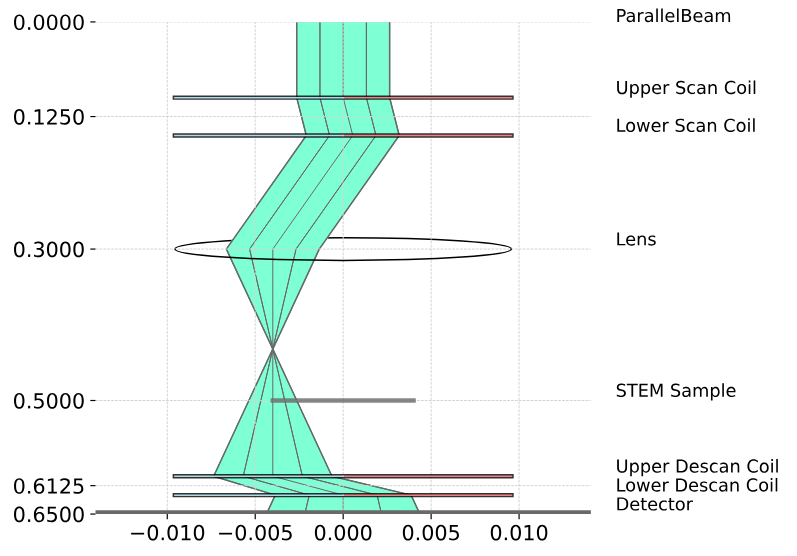
In recent years, ultrafast detectors with high frame rate became available and are used increasingly in practice. These detectors are particularly impactful for scanning transmission electron microscopy (STEM, Figure 1) where the beam is focused, scanned over the specimen, and signals are recorded at each scan position. Detectors with ultrahigh frame rate allow taking an image of the full transmitted beam at each scan position with practical scan speeds. Today, scan speeds beyond 1 Mpix/s with a detector resolution of 512x512 px are reached. This technique is called 4D STEM: Two dimensions for moving the beam over the sample (scan grid) and two dimensions for the detector that images the beam at each position.
It captures a maximum of information from the specimen, and the data can be interpreted with various computational imaging techniques that extract detailed, quantitative information. However, it also generates very large amounts of data, up to 100s of GB per scan, that can be challenging to manage and analyze.
Reproducible, quantitative results from computational imaging techniques require accurately inverting the imaging process to draw conclusions on the specimen. The electron-specimen interaction is complex and the results may change significantly from even minor parameter variations. Therefore, a particularly accurate and precise calibration of the imaging process is necessary. The full description of the electron-optical setup of a TEM requires hundreds of parameters that are not always easy to determine. Since this number of parameters would overwhelm most users, they are presented with abstracted parameters that correspond to a simplified model of the experiment. These parameters are converted to the actual control inputs based on a model of the instrument that has been calibrated at a number of operating points. This model is usually proprietary information of the vendor, not available to the user and not always accurate, in particular when deviating from normal operating points. Developing better and more reliable instrument models and calibration techniques that are correct, open, and interoperable between data analysis techniques and instrument control is becoming an important research field in TEM for that reason.

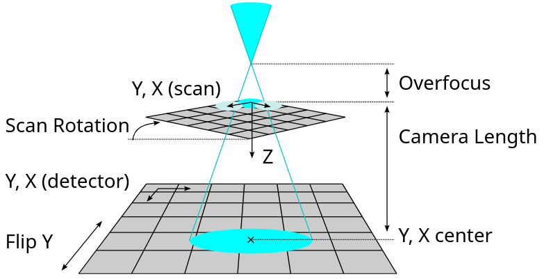
At the ER-C we are working on an interoperable combination of instrument model, metadata schema, calibration methodology, human-machine interface and data analysis to calibrate the fundamental geometry of a 4D STEM experiment (See ref. [1], Figure 2). This includes the scan step, scan direction, focus position, effective camera length (relation between scattering angle and detector pixel position), handedness, and position of the optical axis on the detector. Note how the model in Figure 1 and 2 are different: Figure 1 is closer to the beam path in an actual instrument with pairs of scan and descan coils, while Figure 2 shows a stronger abstraction where the specimen is, effectively, moved relative to the beam. This simplification is suitable for most data analysis. Currently, the calibration technique requires human interaction to achieve a rough calibration. After that is achieved, the parameters can be optimized numerically.
The aim for this project is to determine a good estimate of these parameters from a 4D STEM dataset that was recorded in a strongly defocused state in one step. In this strongly defocused state, the detector receives a shadow image of the specimen from the straight propagation of electrons from the point-like focus through the specimen onto the detector (Figures 1 and 2). The image on the detector shifts as the beam is scanned over the specimen. Consequently, the resulting dataset is a four-dimensional numerical array, where the first two dimensions are the scan dimensions, and the last two dimensions are the detector images that show shifted projections of the specimen.
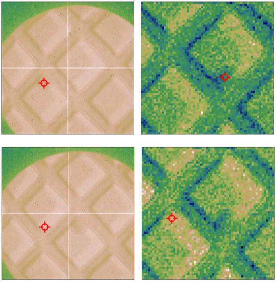
Figure 3 shows plots extracted from such a real-world dataset. In that state, the detector records shadow image projections of a product of the specimen, the beam-limiting aperture, and the detector’s transfer function. When changing the scan position, the projected image of the specimen shifts. The transformation between specimen and detector image is straightforward to simulate with ray tracing [2]. The ground truth for a simulated dataset is known, and for a real dataset it can be determined with the pre-existing manual calibration method. Furthermore, real data can easily be recorded at an instrument with various settings and validated with the pre-existing calibration method.

The task in this project is to develop a machine learning approach that, given a 4D STEM image or a small 4D STEM dataset of images (typical range 16x16x128x128 px to 128x128x512x512 px), can estimate the device parameters (focus, scan rotation, etc., see Figure 2) that are accurate enough to continue with numerical optimization. The aim is to have less than 10% deviation from the ground truth. While some of the input parameters are calibrated beforehand, such as the detector pixel pitch, scan step size and camera length. Others, such as overfocus, scan rotation, and handedness (flip_y) may be erroneous and need to be calibrated. It is necessary to rely on some previously calibrated parameters and not determine all parameters directly since scan step, overfocus, camera length and detector pixel size are collinear, together constituting a single scaling parameter between scan and detector coordinates.
There are two main challenges from a machine learning perspective:
Radboud University: Twan van Laarhoven, Johan Mentink
ER-C Juelich: Dieter Weber, Rafal Dunin-Borkowski
CNR Istituto Nanoscienze (Italy): Enzo Rotunno
[1] https://arxiv.org/abs/2403.08538v1
[2] https://github.com/TemGym/TemGym